Estimation of VO₂max after Nes et al. (2011) – Worked Example
Table of Contents
- Non-Exercise VO₂max Estimation — The Nes (2011) Model
- Applying the Model — Three Worked Examples
- Interpretation & Limitations
1 Non-Exercise VO₂max Estimation — The Nes (2011) Model
Learning objectives:
- The four non-exercise predictors of VO₂peak: age, BMI, resting heart rate and PA-Index
- The sex-specific Nes (2011) equations, their R² and standard error of estimate (SEE)
- Construction and scoring of the Physical Activity Index
1.1 Background
The Nes et al. (2011) model allows non-exercise-based estimation of VO₂peak using only four easily obtainable variables: age, BMI, resting heart rate, and a self-reported physical activity index (PA-Index). The model was developed and validated in the HUNT Study (Nord-Trøndelag Health Study, Norway) with over 4,600 healthy adults.
1.2 Prediction Equations
Men:
VO₂max (ml·kg⁻¹·min⁻¹) = 92.05 − 0.327 × Age − 0.933 × BMI − 0.167 × RHR + 0.257 × PA-IndexR² = 0.59; SEE = 5.8 ml·kg⁻¹·min⁻¹
Women:
VO₂max (ml·kg⁻¹·min⁻¹) = 70.77 − 0.244 × Age − 0.749 × BMI − 0.107 × RHR + 0.213 × PA-IndexR² = 0.57; SEE = 5.1 ml·kg⁻¹·min⁻¹
The four predictors are all physiologically plausible: age and BMI lower predicted fitness, an elevated resting heart rate (RHR) signals reduced cardiovascular fitness, and a higher PA-Index reflects greater habitual activity.
1.3 Physical Activity Index (PA-Index)
The PA-Index is composed of three self-report questions:
Scoring of the three self-report questions that make up the Physical Activity Index (PA-Index).
| Question | Answer | Score |
|---|---|---|
| 1. Frequency — How often do you exercise per week? | Never / less than once | 0 |
| Once per week | 1 | |
| 2–3 times per week | 2 | |
| Almost every day | 3 | |
| 2. Intensity — How hard do you push yourself? | No sweating/heavy breathing | 0 |
| Sweating and heavy breathing | 5 | |
| Push to exhaustion | 10 | |
| 3. Duration — Average training duration per session? | < 15 min or 15–30 min | 1 |
| 30–60 min or > 60 min | 1.5 |
Scoring of the three self-report questions that make up the Physical Activity Index (PA-Index).
PA-Index = Frequency + Intensity + Duration (Range: 1 – 14.5)
Because Intensity carries by far the largest per-answer weight (up to 10 of the 14.5 points), the PA-Index is dominated by how hard a person trains rather than how often or how long. Valid input also depends on standardised measurement of resting heart rate (seated, quiet, ideally morning).
One-Minute-Paper Topics
A One-Minute-Paper (OMP) is a short, focused prompt that students answer in ~60 seconds at the end of a session to consolidate learning, surface misconceptions, and provide formative feedback. When answering, be concise, specific, and use terminology from today’s session.
- Name the four predictor variables in the Nes et al. (2011) model and explain in one sentence why each one is physiologically plausible.
- Read the signs off both equations: which predictors lower the estimate, which one raises it?
- Explain why resting heart rate is included as a negative predictor in the Nes formula — what does an elevated resting HR tell us about cardiovascular fitness?
- Describe the PA-Index: how is it calculated, what is its possible range, and why does its Intensity item carry so much weight?
- Explain why resting-HR measurement conditions (seated, quiet, morning) matter for valid input into the prediction model.
- Describe one scenario in which the PA-Index could systematically overestimate or underestimate actual physical fitness, and what measurement approach would improve accuracy.
Key References
- Nes BM, Janszky I, Vatten LJ, Nilsen TI, Aspenes ST, Wisløff U. Estimating V̇O₂peak from a nonexercise prediction model: the HUNT Study, Norway. Med Sci Sports Exerc 43 (11), 2011: 2024–2030. doi:10.1249/MSS.0b013e31821d3f6f.
2 Applying the Model — Three Worked Examples
Learning objectives:
- Step-by-step VO₂max computation from anthropometric and PA-Index inputs
- Conversion of VO₂max to MET and interpretation against fitness categories
- Comparison of estimates across age, sex and activity profiles
2.1 Worked Example 1: Male Student, 24 Years, Moderately Active
2.1.1 Anthropometric Data
Worked Example 1 — anthropometric input data (24-year-old male).
| Variable | Value |
|---|---|
| Sex | male |
| Age | 24 years |
| Height | 181 cm |
| Body mass | 78 kg |
| BMI | 78 / (1.81)² = 23.8 kg/m² |
| Resting HR (seated) | 68 bpm |
Worked Example 1 — anthropometric input data (24-year-old male).
2.1.2 Physical Activity Index
Worked Example 1 — Physical Activity Index scoring.
| Question | Selected answer | Score |
|---|---|---|
| Frequency | 2–3 times/week | 2 |
| Intensity | Sweating and heavy breathing | 5 |
| Duration | 30–60 min | 1.5 |
Worked Example 1 — Physical Activity Index scoring.
PA-Index = 2 + 5 + 1.5 = 8.5
2.1.3 Estimated VO₂max (Male Formula)
VO₂max = 92.05 − 0.327 × 24 − 0.933 × 23.8 − 0.167 × 68 + 0.257 × 8.5
       = 92.05 − 7.848 − 22.214 − 11.356 + 2.184
       = 52.82 ml·kg⁻¹·min⁻¹  (SEE = ±5.8 ml·kg⁻¹·min⁻¹)

VO₂max in MET = 52.82 / 3.5 = 15.1 MET  (SEE = ±1.7 MET)
Interpretation: A predicted VO₂max of ~53 ml·kg⁻¹·min⁻¹ places this 24-year-old male student in a good-to-excellent fitness category for his age group.
2.2 Worked Example 2: Female Student, 22 Years, Highly Active
2.2.1 Anthropometric Data
Worked Example 2 — anthropometric input data (22-year-old female).
| Variable | Value |
|---|---|
| Sex | female |
| Age | 22 years |
| Height | 168 cm |
| Body mass | 62 kg |
| BMI | 62 / (1.68)² = 22.0 kg/m² |
| Resting HR (seated) | 58 bpm |
Worked Example 2 — anthropometric input data (22-year-old female).
2.2.2 Physical Activity Index
Worked Example 2 — Physical Activity Index scoring.
| Question | Selected answer | Score |
|---|---|---|
| Frequency | Almost every day | 3 |
| Intensity | Push to exhaustion | 10 |
| Duration | > 60 min | 1.5 |
Worked Example 2 — Physical Activity Index scoring.
PA-Index = 3 + 10 + 1.5 = 14.5
2.2.3 Estimated VO₂max (Female Formula)
VO₂max = 70.77 − 0.244 × 22 − 0.749 × 22.0 − 0.107 × 58 + 0.213 × 14.5
       = 70.77 − 5.368 − 16.453 − 6.206 + 3.088
       = 45.83 ml·kg⁻¹·min⁻¹  (SEE = ±5.1 ml·kg⁻¹·min⁻¹)

VO₂max in MET = 45.83 / 3.5 = 13.1 MET  (SEE = ±1.5 MET)
Interpretation: A predicted VO₂max of ~46 ml·kg⁻¹·min⁻¹ places this 22-year-old female student in an excellent fitness category for her age group, consistent with her high training volume.
2.3 Worked Example 3: Older Inactive Male, 55 Years
2.3.1 Anthropometric Data
Worked Example 3 — anthropometric input data (55-year-old male).
| Variable | Value |
|---|---|
| Sex | male |
| Age | 55 years |
| Height | 175 cm |
| Body mass | 92 kg |
| BMI | 92 / (1.75)² = 30.0 kg/m² |
| Resting HR (seated) | 78 bpm |
Worked Example 3 — anthropometric input data (55-year-old male).
2.3.2 Physical Activity Index
Worked Example 3 — Physical Activity Index scoring.
| Question | Selected answer | Score |
|---|---|---|
| Frequency | Less than once/week | 0 |
| Intensity | No sweating | 0 |
| Duration | < 15 min | 1 |
Worked Example 3 — Physical Activity Index scoring.
PA-Index = 0 + 0 + 1.0 = 1.0
2.3.3 Estimated VO₂max (Male Formula)
VO₂max = 92.05 − 0.327 × 55 − 0.933 × 30.0 − 0.167 × 78 + 0.257 × 1.0
       = 92.05 − 17.985 − 28.028 − 13.026 + 0.257
       = 33.27 ml·kg⁻¹·min⁻¹  (SEE = ±5.8 ml·kg⁻¹·min⁻¹)

VO₂max in MET = 33.27 / 3.5 = 9.5 MET  (SEE = ±1.7 MET)
Interpretation: A predicted VO₂max of ~33 ml·kg⁻¹·min⁻¹ reflects the combined effects of higher age, elevated BMI (obesity grade I), higher resting HR, and minimal physical activity. This places the individual in a below-average fitness category.
2.4 Summary Comparison Table
Summary comparison of predicted VO₂max across the three worked examples.
| Parameter | Example 1 | Example 2 | Example 3 |
|---|---|---|---|
| Sex | male | female | male |
| Age (years) | 24 | 22 | 55 |
| BMI (kg/m²) | 23.8 | 22.0 | 30.0 |
| Resting HR (bpm) | 68 | 58 | 78 |
| PA-Index | 8.5 | 14.5 | 1.0 |
| pred. VO₂max (ml·kg⁻¹·min⁻¹) | 52.8 | 45.8 | 33.3 |
| pred. VO₂max (MET) | 15.1 | 13.1 | 9.5 |
Summary comparison of predicted VO₂max across the three worked examples.
One-Minute-Paper Topics
A One-Minute-Paper (OMP) is a short, focused prompt that students answer in ~60 seconds at the end of a session to consolidate learning, surface misconceptions, and provide formative feedback. When answering, be concise, specific, and use terminology from today’s session.
- Convert a predicted VO₂max of 40 ml·kg⁻¹·min⁻¹ to MET and explain what the MET unit represents physiologically.
- Compare the three worked examples (24 y male, 22 y female, 55 y male): which variable combination explains the largest difference between Example 1 and Example 3?
- A 30-year-old woman reports exercising almost every day at exhaustion for >60 min but has a BMI of 31 and a resting HR of 80 bpm. Without calculating, predict whether her VO₂max will be above or below average for her age — and explain your reasoning using the model variables.
- Relate VO₂max to the concept of homeostasis from Lecture 1: how does a higher VO₂max reflect an organism’s improved capacity to regulate homeostasis during aerobic exercise?
- Why might long-term training adaptations (hormesis) increase VO₂max, and which of the four model variables would most visibly reflect these adaptations over a 12-week training programme?
Key References
- Nes BM, Janszky I, Vatten LJ, Nilsen TI, Aspenes ST, Wisløff U. Estimating V̇O₂peak from a nonexercise prediction model: the HUNT Study, Norway. Med Sci Sports Exerc 43 (11), 2011: 2024–2030. doi:10.1249/MSS.0b013e31821d3f6f.
3 Interpretation & Limitations
Learning objectives:
- One-at-a-time sensitivity, and why BMI dominates the estimate
- The SEE prediction band, and why it exceeds the effect of any single predictor
- Equation-vs-person comparison, mean-level strength vs individual-level weakness, and transportability
3.1 Discussion Points
- Which variable has the greatest influence? BMI has the largest regression coefficient (−0.933 for men), followed by resting HR and age. PA-Index has the smallest absolute weight but can range up to 14.5 points.
- Limitations of the model: an R² of ~0.58 means about 42 % of variance is unexplained. An SEE of 5–6 ml·kg⁻¹·min⁻¹ is clinically relevant. The model cannot replace a maximal exercise test for precise measurement.
- Practical application: useful for epidemiological studies and risk stratification in large populations where exercise testing is not feasible (e.g. primary-care screening).
- Comparison with measured values: students can compare their predicted VO₂max with directly measured values from ergospirometry (if available) and discuss the prediction error.
- Sensitivity analysis: what happens if we change only one variable? For example, reducing the resting HR from 78 to 58 in Example 3 would increase predicted VO₂max by 0.167 × 20 = +3.3 ml·kg⁻¹·min⁻¹.
3.2 One-at-a-Time Sensitivity of All Four Predictors
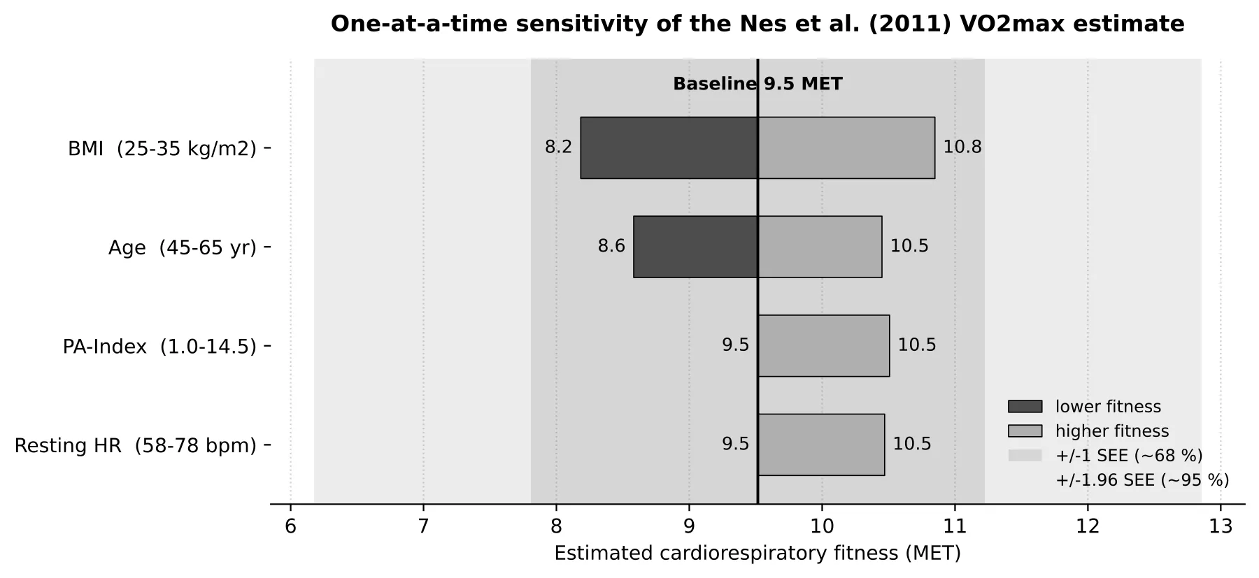
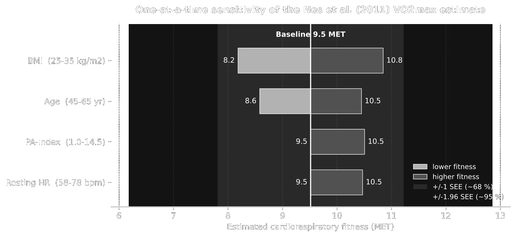
Because the Nes model is an additive linear equation with no interaction terms, each regression coefficient acts as a partial derivative: changing one predictor by a given amount shifts the estimate by a constant rate, independent of the other inputs. The tornado plot below applies this to Worked Example 3 (55 yr male; baseline ≈ 9.5 MET) by varying each predictor across a realistic range while holding the others fixed (resting HR varied from the baseline 78 bpm down to a trained 58 bpm).
One-at-a-time sensitivity of the Nes et al. (2011) VO₂max estimate, shown against the ±1 SEE and ±1.96 SEE prediction bands.
One-at-a-time sensitivity of the Nes et al. (2011) VO₂max estimate, shown against the ±1 SEE and ±1.96 SEE prediction bands.
One-at-a-time sensitivity of each predictor in the Nes model applied to Worked Example 3 (baseline ≈ 9.5 MET).
| Predictor (range varied) | MET range | Effect (MET) |
|---|---|---|
| BMI (25–35 kg/m²) | 8.2 – 10.8 | 2.67 |
| Age (45–65 yr) | 8.6 – 10.5 | 1.87 |
| PA-Index (1.0 – 14.5) | 9.5 – 10.5 | 0.99 |
| Resting HR (58–78 bpm) | 9.5 – 10.5 | 0.95 |
One-at-a-time sensitivity of each predictor in the Nes model applied to Worked Example 3 (baseline ≈ 9.5 MET).
Reading the plot. Bars extending left of the baseline indicate combinations producing lower predicted fitness; bars extending right indicate higher fitness. BMI is by far the most influential single predictor (largest absolute coefficient, −0.933), followed by age. The remaining two bars are one-sided because the baseline subject sits at the unfavourable end of each chosen range — PA-Index at the activity floor (1.0) and resting HR at the top of the 58–78 bpm range (78). Notably, these are also the two modifiable predictors: this individual could gain roughly +1 MET either by becoming maximally active (PA-Index → 14.5) or by lowering resting heart rate to a trained level (78 → 58 bpm). Age and BMI, by contrast, are structural for a given assessment.
3.3 What the SEE Band Represents
The grey strips behind the bars show the model’s own predictive uncertainty, expressed as the Standard Error of Estimate (SEE) — the typical deviation of measured from predicted VO₂max in the validation sample (HUNT: SEE = 5.8 ml·kg⁻¹·min⁻¹ for men, ≈ ±1.7 MET). Interpreted via the normal distribution:
- ±1 SEE (≈ ±1.7 MET) — the darker strip — encloses roughly 68 % of true values around the estimate.
- ±1.96 SEE (≈ ±3.3 MET) — the lighter strip — approximates the ~95 % prediction band for a single new individual.
The decisive teaching point is visible at a glance: every individual predictor bar fits entirely within the ±1 SEE band. Even the most influential variable (BMI, spanning 2.67 MET) moves the point estimate by less than the model’s own ±1 SEE noise. In other words, the measurement uncertainty of the equation is larger than the effect of any single one of its variables.
3.4 Male versus Female: Two Distinct Comparisons
The Nes model uses separate equations for men and women, which invites comparison. Two fundamentally different questions can be asked, and they should not be confused.
3.4.1 Equation Comparison — Same Input, Different Formula
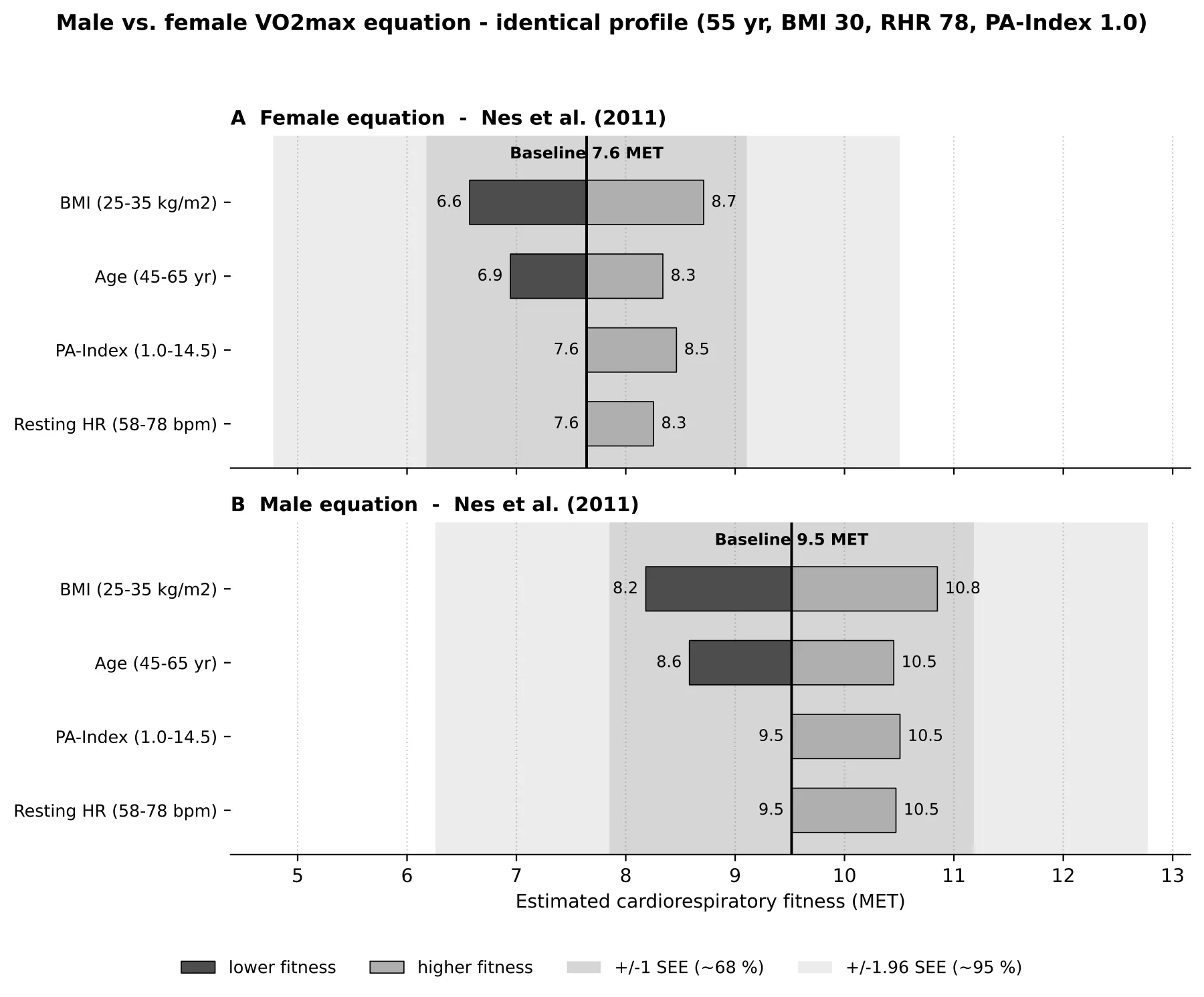
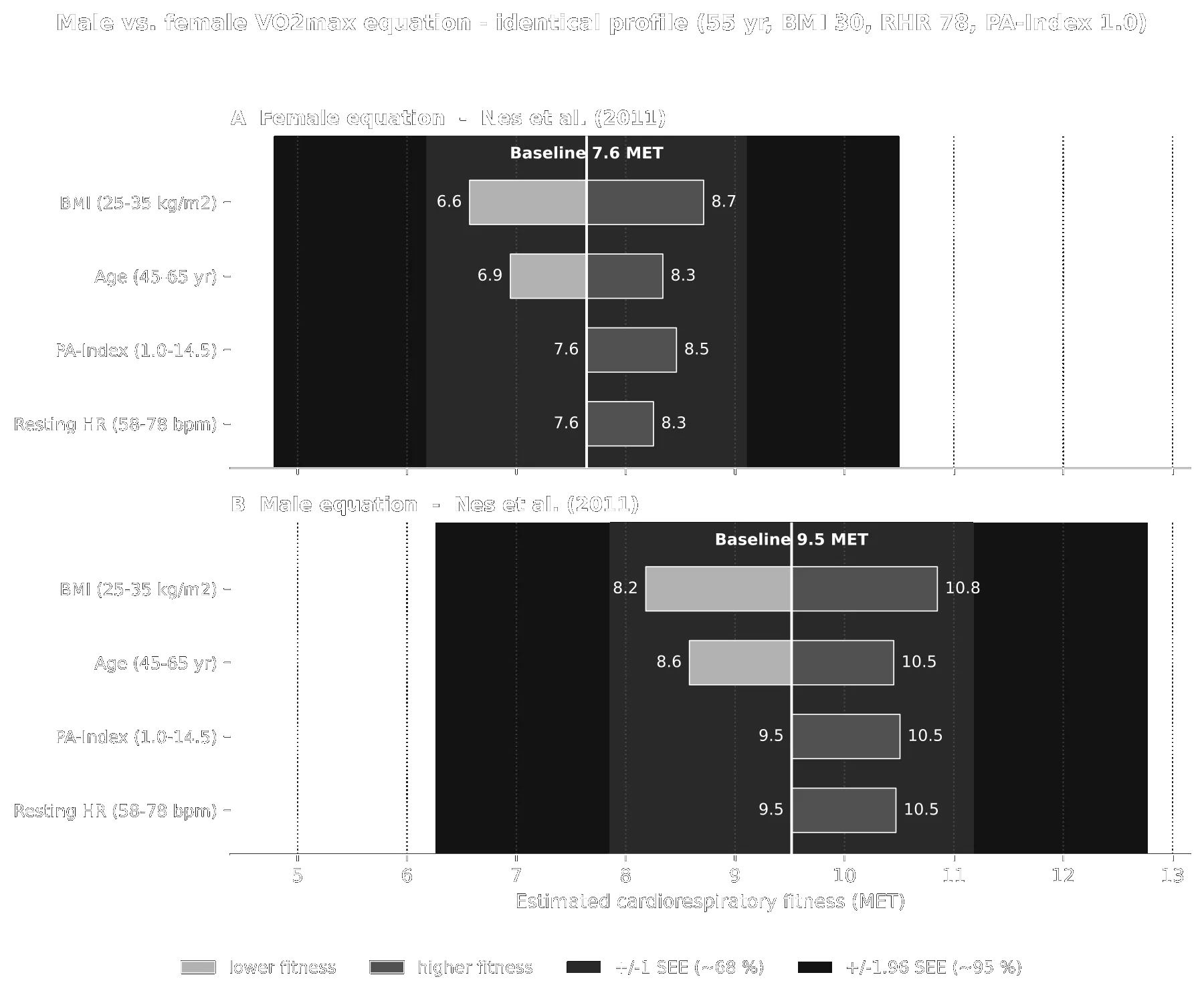
Applying both equations to one identical profile (the Example 3 inputs: 55 yr, BMI 30, RHR 78, PA-Index 1.0) isolates the effect of the equation itself, holding the person constant.
Male vs. female VO₂max equation applied to one identical input profile; bars and SEE bands in greyscale.
Male vs. female VO₂max equation applied to one identical input profile; bars and SEE bands in greyscale.
Two features stand out. First, a level difference: the female equation returns ≈ 7.6 MET versus ≈ 9.5 MET for the same profile (Δ ≈ 1.9 MET), driven almost entirely by the lower intercept (70.77 vs 92.05) and reflecting the generally lower VO₂max of women at equal body build. Second, lower sensitivity: because every female coefficient is smaller in absolute value, each female bar is shorter than its male counterpart (e.g. BMI 2.1 vs 2.7 MET). With baseline and ranges held identical, bar length here equals coefficient × range, so the difference is purely a coefficient effect.
3.4.2 Person Comparison — Different People, Each with Their Own Equation
Comparing the two actual worked examples keeps each individual’s real profile and sex-specific equation. This answers a clinically realistic question but confounds sex, age, body composition, and activity.
Person comparison of Example 2 (fit young female) and Example 3 (inactive older male), each with own profile and equation.
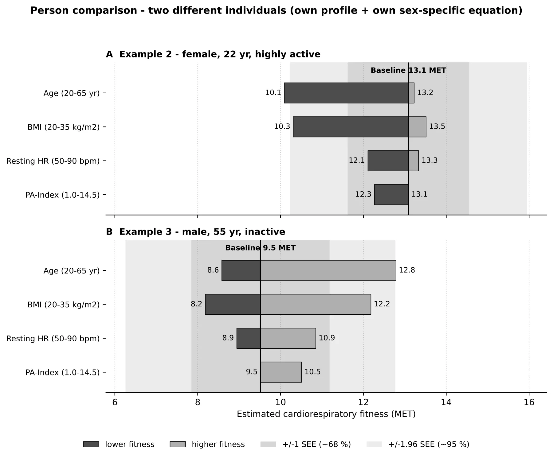
Person comparison of Example 2 (fit young female) and Example 3 (inactive older male), each with own profile and equation.
Here the contrast is one of position in the predictor space. The fit 22-year-old woman sits near a ceiling (baseline ≈ 13.1 MET): most bars extend leftward, i.e. realistic changes can almost only lower her estimate. The inactive 55-year-old man sits near a floor (≈ 9.5 MET): his bars extend rightward, i.e. almost any change improves the estimate. The same predictor can therefore be “protective” or “modifiable” depending solely on where the individual starts.
Bottom line for teaching. Use the comparison in §3.4.1 to explain why the equations differ; use the comparison in §3.4.2 to explain why two real people differ. Bar length reflects both the regression coefficient (§3.4.1) and the subject’s position within the varied range (§3.4.2), and the two contributions must be read separately.
3.5 The Mean versus the Individual
Non-exercise prediction equations estimate maximal oxygen uptake from readily available demographic and physiological variables without a maximal or submaximal exercise test. Derived by multiple linear regression, they yield an additive, interaction-free approximation whose precision is summarised by the SEE.
At the level of the group mean, the approach is a genuine strength. Because regression returns an unbiased estimate of the conditional mean, population and subgroup averages are recovered accurately at negligible cost and risk. This makes non-exercise equations well suited to epidemiological surveillance, large-scale screening, and group-level risk stratification, where no ergometry, no maximal effort, and no specialised equipment are required — a decisive advantage in clinical or deconditioned populations for whom maximal testing is contraindicated.
At the level of the individual, the same equation is comparatively weak. The wide SEE means the prediction interval for a single person spans several MET — here wider than the effect of realistically varying any single predictor. Individual fitness classification is therefore uncertain, particularly near category boundaries, and estimates are subject to regression toward the sample mean, so that truly high- and low-fit individuals are systematically under- and over-estimated. Surrogate predictors (notably BMI standing in for body composition) further limit individual validity in non-representative groups such as athletes or older adults.
A third caveat is transportability: the equation was developed in 4,600+ Norwegian HUNT participants. Applied to a systematically different population (e.g. elite athletes, other ethnicities, the very old), even the mean estimate may be biased — this is a validity problem, not an SEE problem.
Take-home message:
Non-exercise equations estimate the average well and the individual poorly. They are appropriate for describing and comparing populations, but point estimates should not be over-interpreted for individual diagnosis, exercise prescription, or longitudinal monitoring, where direct or submaximal measurement remains preferable.
One-Minute-Paper Topics
A One-Minute-Paper (OMP) is a short, focused prompt that students answer in ~60 seconds at the end of a session to consolidate learning, surface misconceptions, and provide formative feedback. When answering, be concise, specific, and use terminology from today’s session.
- The BMI coefficient is the largest in absolute terms (−0.933 for men). Why does higher BMI reduce predicted VO₂max even if the individual exercises regularly?
- Compare the male and female prediction equations: which variable shows the greatest sex-specific difference in its regression coefficient, and what might explain this?
- The model has an R² of ~0.58. What does this mean for individual-level interpretation, and what does the unexplained 42 % of variance likely represent?
- Define SEE (Standard Error of Estimate) and explain what it means in practice if the SEE for men is ±5.8 ml·kg⁻¹·min⁻¹.
- Name two populations or contexts in which a non-exercise estimation of VO₂max would be preferred over a direct maximal exercise test, and justify your answer.
- The model was developed and validated in the HUNT Study with over 4,600 Norwegian adults. Identify one potential limitation when applying it to a different population (e.g. elite athletes or clinical patients).
- Explain what “sensitivity analysis” means in the context of the Nes model, and give one concrete numerical example from the lecture of how changing a single variable shifts the predicted VO₂max.
- Which concept from today’s session was most counter-intuitive or surprising to you, and why?
- What single question about VO₂max estimation, model limitations, or the practical application of the Nes formula would you most like answered in the next lecture?
Key References
- Nes BM, Janszky I, Vatten LJ, Nilsen TI, Aspenes ST, Wisløff U. Estimating V̇O₂peak from a nonexercise prediction model: the HUNT Study, Norway. Med Sci Sports Exerc 43 (11), 2011: 2024–2030. doi:10.1249/MSS.0b013e31821d3f6f.
References
- Nes BM, Janszky I, Vatten LJ, Nilsen TI, Aspenes ST, Wisløff U. Estimating V̇O₂peak from a nonexercise prediction model: the HUNT Study, Norway. Med Sci Sports Exerc 43 (11), 2011: 2024–2030. doi:10.1249/MSS.0b013e31821d3f6f.